Statistics
Contents
8. Statistics#
Considering the amount of data produced nowadays in many fields, the computer manipulation of this information is not only important but also has become a very active field of study. Despite of the fact of increasing computational facilities, the effort necessary to make statistical analysis has become more complicated, at least in the computational aspect. This is why becomes fundamental to some aspects, leastwise in a raw way.
Contents
%pylab inline
%pylab is deprecated, use %matplotlib inline and import the required libraries.
Populating the interactive namespace from numpy and matplotlib
import numpy as np
from matplotlib import animation
https://drive.google.com/file/d/12cwfl5i2SVlNF60oUF9-ep3q7NHB4AcH/view?usp=sharing### Data Adjust See also:
https://www.mathsisfun.com/data/least-squares-regression.html
http://blog.mmast.net/least-squares-fitting-numpy-scipy
https://stackoverflow.com/a/43623588/2268280
Given a data set, the first approach to find a function that passes through the points would be using a interpolation polynomial. But we should take special attention to the way data set is gathered, i.e., usually is a sample obtained experimentally or in a way that has associated an intrinsic error. Then, forcing that the approximate function passes through all the points would actually incur in incrementing the error. This is why it is necessary to build a different procedure to build the function that fits the data.
The fitting functions, though, are build using a Lagrange polynomial and the order of this polynomial constitutes the approximation that is going to be used. But the fitting function is not going to take the exact value in the known points, they are going to desagree in certain tolerance value.
8.1. Linear least squares#
Approximating a data set to a linear Langrange polynomial would be just to use $\( y_i= f(x_i) = a_1x_i + a_0\,. \)\( However, with experimental data, the problem is that the values \)y_i\( are not precise, then it is proposed to find the best approximation. For the best _linear approximation_, we need to find for _all_ points the value of \)a_0\( and \)a_1\( that _minimize_ the error \)\( E = E(a_0,a_1) = \sum_{i=1}^{m}[y_i - (a_1 x_i + a_0)]^2 \)$ where the square is more well suited for the minimization procedure since avoids the fluctions for changes of sign.
To minimize the function of 2 variables, \(E(a_0,a_1)\) with respect to \(a_0\) and \(a_1\), it is necessary to set its partial derivatives to zero and simultaneously solve to the resulting equations.
To establish the minimzation equations, it is necesary to take the partial derivatives with respect to \(a_0\) and \(a_1\) and and equal them to zero $\( \frac{\partial E}{\partial a_0} = 0\,, \hspace{1cm} \frac{\partial E}{\partial a_1} = 0\,. \)$
Afterwards,
Replacing back in the second equation
Therefore
Replacing back in \(a_0\)
where the coefficients \(a_0\) and \(a_1\) can be easily obtained
Now, using the error definition one can find the error associated to the approximation made,
since the coefficients \(a_0\) and \(a_1\) are already known.
From Least square method in python:
There are many curve fitting functions in scipy and numpy and each is used differently, e.g. scipy.optimize.leastsq and scipy.optimize.least_squares. For simplicity, we will use scipy.optimize.curve_fit, but it is difficult to find an optimized regression curve without selecting reasonable starting parameters. A simple technique will later be demonstrated on selecting starting parameters.
In our first example the starting parameters will be just zeros
8.1.1. Example 1#
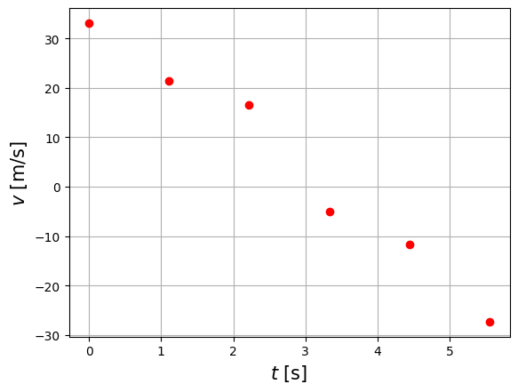
A body is moving under the influence of an external force, the variation of the position measured for different times are compiled in table 1
t(s) |
x(m) |
v(m/s) |
|---|---|---|
0 |
2.76 |
33.10 |
1.11 |
29.66 |
21.33 |
2.22 |
46.83 |
16.57 |
3.33 |
44.08 |
-5.04 |
4.44 |
37.26 |
-11.74 |
5.55 |
12.03 |
-27.32 |
%pylab inline
%pylab is deprecated, use %matplotlib inline and import the required libraries.
Populating the interactive namespace from numpy and matplotlib
import pandas as pd
#'x': [2.76,  29.66,46.83,44.08,37.26,12.03],
df=pd.DataFrame( {'t': [ 0.,  1.11,  2.22,  3.33,  4.44, 5.55],#'x': [2.76,  29.66,46.83,44.08,37.26,12.03],
                  'v': [33.10, 21.33, 16.57, -5.04, -11.74, -27.32]} )
df[['t','v']]
| t | v | |
|---|---|---|
| 0 | 0.00 | 33.10 |
| 1 | 1.11 | 21.33 |
| 2 | 2.22 | 16.57 |
| 3 | 3.33 | -5.04 |
| 4 | 4.44 | -11.74 |
| 5 | 5.55 | -27.32 |
plt.plot(df.t,df.v,'ro')
plt.xlabel('$t$ [s]',size=15 )
plt.ylabel('$v$ [m/s]',size=15 )
plt.grid()
import scipy.optimize as optimize
def func(t,a1,a0):
    return a1*t+a0
The starting point is optional
starting_parameters=[0,0]
a,Δa=optimize.curve_fit(func,df.t,df.v,p0=starting_parameters)
a
array([-10.88597169, 34.69190478])
The correlation matrix,\(\Delta a\) , give as the error in the determination of the parameters
Δa
array([[ 0.68398817, -1.89806718],
       [-1.89806718,  7.72513347]])
np.diag(Δa)
array([0.68398817, 7.72513347])
print(a)
print('-'*20)
print(Δa)
σ = np.sqrt(np.diag(Δa))
print('-'*20)
print('a1={:.2f}±{:.2f}, a0={:.1f}±{:.1f}'.format(a[0],σ[0],a[1],σ[1]) )
[-10.88597169  34.69190478]
--------------------
[[ 0.68398817 -1.89806718]
 [-1.89806718  7.72513347]]
--------------------
a1=-10.89±0.83, a0=34.7±2.8
t_lin=np.linspace(0,5.55)
v_model=func(t_lin,*a) #func(t_lin,a[0],a[1])
df['v_fitted']=func(df.t,*a)
df
| t | v | v_fitted | |
|---|---|---|---|
| 0 | 0.00 | 33.10 | 34.691905 |
| 1 | 1.11 | 21.33 | 22.608476 |
| 2 | 2.22 | 16.57 | 10.525048 |
| 3 | 3.33 | -5.04 | -1.558381 |
| 4 | 4.44 | -11.74 | -13.641810 |
| 5 | 5.55 | -27.32 | -25.725238 |
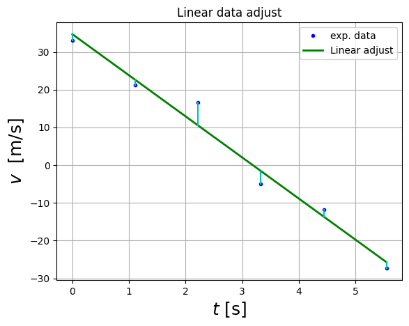
plt.plot(df.t,df.v,'b.',label='exp. data')
plt.plot(df.t,a[0]*df.t+a[1],'g-',lw=2,label="Linear adjust")
for i in range(df.t.size):
    plt.plot(np.array([df.t[i],df.t[i]]), np.array([df.v[i],df.v_fitted[i] ]),"c-")

plt.xlabel( "$t$ [s]", fontsize = 18 )
plt.ylabel( "$v$  [m/s]", fontsize = 18 )
plt.title("Linear data adjust")
plt.legend()
plt.grid()
Activity: plot the error bands. Use https://beta.deepnote.com/project/4b6ea05f-f155-4eae-959c-cd064deaa7b6
Activity: Solve the problem with fmin_powell for the fit only (not the error correlation matrix)
$\(
E = E(a_0,a_1) = \sum_{i=1}^{m}[y_i - (a_1 x_i + a_0)]^2
\)$
Solution: Let a=[a_0,a_1]
def E(a,x=df.t.values,y=df.v.values):
    return ((y-(a[1]*x+a[0]))**2).sum()
E([1,0])
2686.9554000000003
E([2,1])
3105.6670999999997
E([33,-10])
79.44340000000005
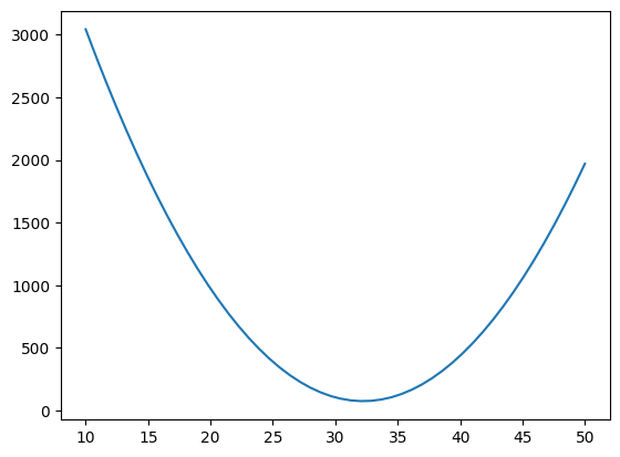
def Ea0(x,a1=-10):
    EE=[]
    for a0 in x:
        EE.append( E([a0,a1]))
    return np.array(EE)
Ea0([2,3])
array([5560.2434, 5203.4434])
a0=np.linspace(10,50)
plt.plot(a0,Ea0(a0,-10))
[<matplotlib.lines.Line2D at 0x7fa1570718e0>]
optimize.fmin_powell(E,[0,0],full_output=True)
Optimization terminated successfully.
         Current function value: 58.991928
         Iterations: 5
         Function evaluations: 169
(array([ 34.69190471, -10.88597167]),
 58.99192761904762,
 array([[ 9.58580558, -2.62474386],
        [ 0.03589244,  0.0271459 ]]),
 5,
 169,
 0)
8.1.2. How does this work:#
From Least sqaure method in python:
curve_fit is one of many optimization functions offered by scipy. Given an initial value, the resulting estimated parameters are iteratively refined so that the resulting curve minimizes the residual error, or difference between the fitted line and sampling data. A better guess reduces the number of iterations and speeds up the result. With these estimated parameters for the fitted curve, one can now calculate the specific coefficients for a particular equation (a final exercise left to the OP).
8.2. Example: Least Action#
Least_action_minimization.ipynb
8.3. Non-linear least square#
In general, it can be used any polynomial order to adjust a data set, since it is satisfied that \(n<m-1\), with n the order of the polynomial and m the number of points known. Then, we have $\( P_n(x) = a_nx^n + a_{n-1}x^{n-1}+...+a_1x+a_0 \)$
Using a similar procedure followed in linear least square approximation, it is chose the constants \(a_0,...a_n\) to minimize the least square error
Expanding the square difference and taking into account that E to be minimized requires that \(\partial E/ \partial a_j = 0 \) for each \(j=0,1,...n\). Following these arguments, it is found that the n+1 equations needed to solve to find the coefficients \(a_j\) are
for each \(j=0,1,...n\). A better way to show the equations, where m is the data length and n is the polynomial order, is
Again, the error associated to the approximation can be obtained by initial definition of E. The error can also be defined using a weight function \(W_i\) as
this function \(W_i\) can be defined in several ways. If \(W_i = \sigma_i\), i.e., the standard deviation per point, \(y_i\pm \sigma_i\), it is necessary to know the probability distribution followed by the experiments. In these cases where it is not known, it is usually taken as one.
8.3.1. Activity #
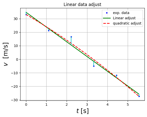
Adjust the position column data in the table 1 to a second order polynomial. What is the acceleration suffered by the body?from scipy import optimize
def func(t,a2,a1,a0):
    return a2*t**2+a1*t+a0
a,kk=optimize.curve_fit(func,df.t,df.v)
t_lin=np.linspace(0,5.55)
v2_model=func(t_lin,*a)
df['v2_fitted']=func(df.t,*a)
df
| t | v | v_fitted | v2_fitted | |
|---|---|---|---|---|
| 0 | 0.00 | 33.10 | 34.691905 | 33.096072 |
| 1 | 1.11 | 21.33 | 22.608476 | 22.927643 |
| 2 | 2.22 | 16.57 | 10.525048 | 11.801714 |
| 3 | 3.33 | -5.04 | -1.558381 | -0.281715 |
| 4 | 4.44 | -11.74 | -13.641810 | -13.322643 |
| 5 | 5.55 | -27.32 | -25.725238 | -27.321071 |
plt.plot(df.t,df.v,'b.',label='exp. data')
plt.plot(t_lin,v_model,'g-',lw=2,label="Linear adjust")
plt.plot(t_lin,v2_model,'r--',lw=2,label="quadratic adjust")
for i in range(df.t.size):
    plt.plot(np.array([df.t[i],df.t[i]]), np.array([df.v[i],df.v_fitted[i] ]),"c-")

plt.xlabel( "$t$ [s]", fontsize = 18 )
plt.ylabel( "$v$  [m/s]", fontsize = 18 )
plt.title("Linear data adjust")
plt.legend()
plt.grid(1)
8.3.2. Activity #
The air drag for a sphere that is moving at high speeds can be expresed in the following form $$ f_{drag} = -\frac{1}{2} C \rho A v^2 $$where C is the drag coefficient(0.5 for a sphere), \(\rho\) is the air density (1.29kg/\(m^3\)) and A is the cross-sectional area. Generate points that have a bias of the value obtanied with \(f_{drag}\) using np.random.random.
Afterwards, use a second order polynomial to fit the data generated and find the error associated to the approximation.
import scipy.optimize as optimize
8.4. Fit to a non-linear function#
Determinar: \(A,c,d\)
import pandas as pd
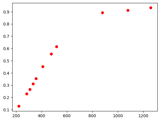
T_values = np.array([222, 284, 308.5, 333, 358, 411, 477, 518, 880, 1080, 1259])
C_values = np.array([0.1282, 0.2308, 0.2650, 0.3120 , 0.3547, 0.4530, 0.5556, 0.6154, 0.8932, 0.9103, 0.9316])

x_samp = T_values
y_samp = C_values
plt.plot(x_samp,y_samp,'ro')
[<matplotlib.lines.Line2D at 0x7f755b7a3bb0>]
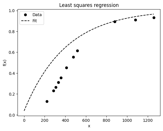
def func(x, A, c, d):
    return A*np.exp(c*x) + d
## REGRESSION ------------------------------------------------------------------
p0 = [0, -3e-2, 1]                                        ## guessed params
w, _ = optimize.curve_fit(func, x_samp, y_samp, p0=p0)
print("E]stimated Parameters", w)

## Model
x_lin=np.linspace(200,1350)
y_model = func(x_lin, *w)
E]stimated Parameters [-1.66301124 -0.0026884 1.0099538 ]
x_lin = np.linspace(0, x_samp.max(), 50)                   ## 50 evenly spaced digits between 0 and max
## PLOT ------------------------------------------------------------------------
## Visualize data and fitted curves
plt.plot(x_samp, y_samp, "ko", label="Data")
plt.plot(x_lin, y_model, "k--", label="Fit")
plt.title("Least squares regression")
plt.legend(loc="upper left")
plt.xlabel('x')
plt.ylabel('f(x)')
Text(0, 0.5, 'f(x)')
import time
for i in range(100):
    time.sleep(0.1)
    if i%10==0:
        print(i,end='\r')
90
8.4.1. Example: exponential fit#
8.4.2. Guess the number of pages of a book#
https://docs.google.com/forms/d/e/1FAIpQLSeZJ0QII5JcST-M9_JgGYNzX3GahULVVFc31DQnWjJ4SdUQwg/viewform?fbclid=IwAR0wEadM0ZH-HXmp3lkAM3emCDPxs_6F509BS3EkOvldp-NFzbCOkZVSjR4
where \(a\) is the height of the gaussian, \(\mu\) is the mean (expected value), and \(\sigma\) es la varianze
import pandas as pd
df=pd.read_csv('https://docs.google.com/spreadsheets/d/e/2PACX-1vTu_XE2dAiTcjHTfbaVKt7xEl_GnNeF_VYFsIBi5uM-gqBlBRfNHso-X1z3lxV7IW2f9UYKmZkSOYv-/pub?output=csv')
---------------------------------------------------------------------------
HTTPError                                 Traceback (most recent call last)
Cell In [55], line 1
----> 1 df=pd.read_csv('https://docs.google.com/spreadsheets/d/e/2PACX-1vTu_XE2dAiTcjHTfbaVKt7xEl_GnNeF_VYFsIBi5uM-gqBlBRfNHso-X1z3lxV7IW2f9UYKmZkSOYv-/pub?output=csv')

File /usr/local/lib/python3.9/dist-packages/pandas/util/_decorators.py:211, in deprecate_kwarg.<locals>._deprecate_kwarg.<locals>.wrapper(*args, **kwargs)
    209     else:
    210         kwargs[new_arg_name] = new_arg_value
--> 211 return func(*args, **kwargs)

File /usr/local/lib/python3.9/dist-packages/pandas/util/_decorators.py:317, in deprecate_nonkeyword_arguments.<locals>.decorate.<locals>.wrapper(*args, **kwargs)
    311 if len(args) > num_allow_args:
    312     warnings.warn(
    313         msg.format(arguments=arguments),
    314         FutureWarning,
    315         stacklevel=find_stack_level(inspect.currentframe()),
    316     )
--> 317 return func(*args, **kwargs)

File /usr/local/lib/python3.9/dist-packages/pandas/io/parsers/readers.py:950, in read_csv(filepath_or_buffer, sep, delimiter, header, names, index_col, usecols, squeeze, prefix, mangle_dupe_cols, dtype, engine, converters, true_values, false_values, skipinitialspace, skiprows, skipfooter, nrows, na_values, keep_default_na, na_filter, verbose, skip_blank_lines, parse_dates, infer_datetime_format, keep_date_col, date_parser, dayfirst, cache_dates, iterator, chunksize, compression, thousands, decimal, lineterminator, quotechar, quoting, doublequote, escapechar, comment, encoding, encoding_errors, dialect, error_bad_lines, warn_bad_lines, on_bad_lines, delim_whitespace, low_memory, memory_map, float_precision, storage_options)
    935 kwds_defaults = _refine_defaults_read(
    936     dialect,
    937     delimiter,
   (...)
    946     defaults={"delimiter": ","},
    947 )
    948 kwds.update(kwds_defaults)
--> 950 return _read(filepath_or_buffer, kwds)

File /usr/local/lib/python3.9/dist-packages/pandas/io/parsers/readers.py:605, in _read(filepath_or_buffer, kwds)
    602 _validate_names(kwds.get("names", None))
    604 ## Create the parser.
--> 605 parser = TextFileReader(filepath_or_buffer, **kwds)
    607 if chunksize or iterator:
    608     return parser

File /usr/local/lib/python3.9/dist-packages/pandas/io/parsers/readers.py:1442, in TextFileReader.__init__(self, f, engine, **kwds)
   1439     self.options["has_index_names"] = kwds["has_index_names"]
   1441 self.handles: IOHandles | None = None
-> 1442 self._engine = self._make_engine(f, self.engine)

File /usr/local/lib/python3.9/dist-packages/pandas/io/parsers/readers.py:1729, in TextFileReader._make_engine(self, f, engine)
   1727     is_text = False
   1728     mode = "rb"
-> 1729 self.handles = get_handle(
   1730     f,
   1731     mode,
   1732     encoding=self.options.get("encoding", None),
   1733     compression=self.options.get("compression", None),
   1734     memory_map=self.options.get("memory_map", False),
   1735     is_text=is_text,
   1736     errors=self.options.get("encoding_errors", "strict"),
   1737     storage_options=self.options.get("storage_options", None),
   1738 )
   1739 assert self.handles is not None
   1740 f = self.handles.handle

File /usr/local/lib/python3.9/dist-packages/pandas/io/common.py:714, in get_handle(path_or_buf, mode, encoding, compression, memory_map, is_text, errors, storage_options)
    711     codecs.lookup_error(errors)
    713 ## open URLs
--> 714 ioargs = _get_filepath_or_buffer(
    715     path_or_buf,
    716     encoding=encoding,
    717     compression=compression,
    718     mode=mode,
    719     storage_options=storage_options,
    720 )
    722 handle = ioargs.filepath_or_buffer
    723 handles: list[BaseBuffer]

File /usr/local/lib/python3.9/dist-packages/pandas/io/common.py:364, in _get_filepath_or_buffer(filepath_or_buffer, encoding, compression, mode, storage_options)
    362 ## assuming storage_options is to be interpreted as headers
    363 req_info = urllib.request.Request(filepath_or_buffer, headers=storage_options)
--> 364 with urlopen(req_info) as req:
    365     content_encoding = req.headers.get("Content-Encoding", None)
    366     if content_encoding == "gzip":
    367         # Override compression based on Content-Encoding header

File /usr/local/lib/python3.9/dist-packages/pandas/io/common.py:266, in urlopen(*args, **kwargs)
    260 """
    261 Lazy-import wrapper for stdlib urlopen, as that imports a big chunk of
    262 the stdlib.
    263 """
    264 import urllib.request
--> 266 return urllib.request.urlopen(*args, **kwargs)

File /usr/lib/python3.9/urllib/request.py:214, in urlopen(url, data, timeout, cafile, capath, cadefault, context)
    212 else:
    213     opener = _opener
--> 214 return opener.open(url, data, timeout)

File /usr/lib/python3.9/urllib/request.py:523, in OpenerDirector.open(self, fullurl, data, timeout)
    521 for processor in self.process_response.get(protocol, []):
    522     meth = getattr(processor, meth_name)
--> 523     response = meth(req, response)
    525 return response

File /usr/lib/python3.9/urllib/request.py:632, in HTTPErrorProcessor.http_response(self, request, response)
    629 ## According to RFC 2616, "2xx" code indicates that the client's
    630 # request was successfully received, understood, and accepted.
    631 if not (200 <= code < 300):
--> 632     response = self.parent.error(
    633         'http', request, response, code, msg, hdrs)
    635 return response

File /usr/lib/python3.9/urllib/request.py:555, in OpenerDirector.error(self, proto, *args)
    553     http_err = 0
    554 args = (dict, proto, meth_name) + args
--> 555 result = self._call_chain(*args)
    556 if result:
    557     return result

File /usr/lib/python3.9/urllib/request.py:494, in OpenerDirector._call_chain(self, chain, kind, meth_name, *args)
    492 for handler in handlers:
    493     func = getattr(handler, meth_name)
--> 494     result = func(*args)
    495     if result is not None:
    496         return result

File /usr/lib/python3.9/urllib/request.py:747, in HTTPRedirectHandler.http_error_302(self, req, fp, code, msg, headers)
    744 fp.read()
    745 fp.close()
--> 747 return self.parent.open(new, timeout=req.timeout)

File /usr/lib/python3.9/urllib/request.py:523, in OpenerDirector.open(self, fullurl, data, timeout)
    521 for processor in self.process_response.get(protocol, []):
    522     meth = getattr(processor, meth_name)
--> 523     response = meth(req, response)
    525 return response

File /usr/lib/python3.9/urllib/request.py:632, in HTTPErrorProcessor.http_response(self, request, response)
    629 ## According to RFC 2616, "2xx" code indicates that the client's
    630 # request was successfully received, understood, and accepted.
    631 if not (200 <= code < 300):
--> 632     response = self.parent.error(
    633         'http', request, response, code, msg, hdrs)
    635 return response

File /usr/lib/python3.9/urllib/request.py:561, in OpenerDirector.error(self, proto, *args)
    559 if http_err:
    560     args = (dict, 'default', 'http_error_default') + orig_args
--> 561     return self._call_chain(*args)

File /usr/lib/python3.9/urllib/request.py:494, in OpenerDirector._call_chain(self, chain, kind, meth_name, *args)
    492 for handler in handlers:
    493     func = getattr(handler, meth_name)
--> 494     result = func(*args)
    495     if result is not None:
    496         return result

File /usr/lib/python3.9/urllib/request.py:641, in HTTPDefaultErrorHandler.http_error_default(self, req, fp, code, msg, hdrs)
    640 def http_error_default(self, req, fp, code, msg, hdrs):
--> 641     raise HTTPError(req.full_url, code, msg, hdrs, fp)

HTTPError: HTTP Error 404: Not Found
df['Guess']=df.Guess.str.replace(',','').astype(int)
bins=range(0,1500,100)
See solution: gaussian_fit.ipynb
See fit exponential: https://github.com/restrepo/COVID-19
import pandas as pd
DataSource='https://raw.githubusercontent.com/CSSEGISandData/COVID-19/'
DataFile='master/csse_covid_19_data/csse_covid_19_time_series/time_series_covid19_confirmed_global.csv'
cva=pd.read_csv('{}{}'.format(DataSource,DataFile))
cva=cva.reset_index(drop=True)
#Special cases
c='Hong Kong'
try:
    cva.loc[cva[cva['Province/State']==c].index[0],'Country/Region']=c
except IndexError:
    pass
def index_field(df,column,filter=None):
    '''
    WARNING: Nonumerical columns are dropped

    Parameters:
    ----------
    filter: list, default None
        Select only the columns in this list
    '''
    dff=df.copy()
    if filter:
        dff=df[[column]+list(filter)]
    return dff.groupby(column).sum()

d=[ c for c in cva.columns if re.search(r'^[0-9]{1,2}\/[0-9]{1,2}\/[1920]{2}',c)]
cv=index_field(cva,"Country/Region",filter=d)
8.5. Random Numbers#
%pylab inline
%pylab is deprecated, use %matplotlib inline and import the required libraries.
Populating the interactive namespace from numpy and matplotlib
In nature it is not uncommon finding phenomena that are random intrinsic, this is why it becomes a necessity to produce random numbers in order to model such events. But, let us think about the operations that a computer can do, they are done following certain stablished rules, how then can be generated random numbers?
This is achieved until certain point, it is only possible produce pseudo numbers, i.e, numbers obtained following some basic rules. At sequence of numbers apparently random but that are going to repeat after some period.
Now, the most basic way to understand the generation of a pseudo-random number consists in following the next recurrence rule that produces integer random numbers
\(r_i\) is the seed, \(a\) and \(b\) and \(N\) are coefficients chose. Notice that \(\%\) represents the module, then the numbers obtained are going to be smaller than N.
Now, consider the case when \( a= 3 \), \(b = 2\) and \(N = 10\) and the initial seed \(r_0 = 3\). The new seed is the number obtaine in the last step.
%pylab inline
%pylab is deprecated, use %matplotlib inline and import the required libraries.
Populating the interactive namespace from numpy and matplotlib
import numpy as np
## Randon number function
def random_number(seed,a=4,b=1,N=9):
    return (a*seed + b)%N

#Constant values
a = 3
b = 2
N = 10
#Amount of random numbers
N_iter = 15
rnumber = np.zeros(N_iter+1)
#Initial seed
rnumber[0] = 4
#rnumber[0] = 10

for i in range(N_iter):
    print(i)
    rnumber[i+1] = random_number(seed=rnumber[i],a=3,b=2,N=10)

print ("Random numbers produced using a = %d, b = %d and N = %d\n" % ( a,b,N ))
print (rnumber[1:])
0
1
2
3
4
5
6
7
8
9
10
11
12
13
14
Random numbers produced using a = 3, b = 2 and N = 10

[4. 4. 4. 4. 4. 4. 4. 4. 4. 4. 4. 4. 4. 4. 4.]
rnumber
array([4., 4., 4., 4., 4., 4., 4., 4., 4., 4., 4., 4., 4., 4., 4., 4.])
x=[]
x.append( random_number(seed=2,a=3,b=2,N=10) )
x
[8]
x.append( random_number(seed=x[0],a=3,b=2,N=10) )
x
[8, 6]
x.append( random_number(seed=x[1],a=3,b=2,N=10) )
x
[8, 6, 0]
x.append( random_number(seed=x[2],a=3,b=2,N=10) )
x
[8, 6, 0, 2]
import random
import numpy as np
import time
print( time.time() )
time.sleep(2)
print( time.time() )
1666895594.8727255
1666895596.8751295
t=time.time()
t/3600/24/365 #s → h → dias → años
52.85691862843985
random.seed(666)
random.random() #seed is unix time
0.9033231539802643
x=random.seed(4890098)
(random.random(),
random.random(),
random.random())
(0.6771981606438447, 0.7282646242796362, 0.12733022922307846)
np.random.random(5)
array([0.24322603, 0.97041503, 0.65472299, 0.94004507, 0.3412584 ])
np.random.seed(2)
np.random.random(5)
array([0.4359949 , 0.02592623, 0.54966248, 0.43532239, 0.4203678 ])
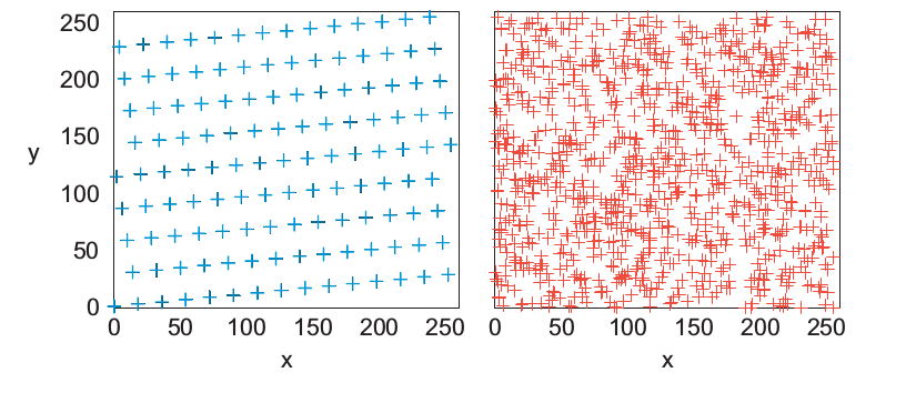
Notice that after N random numbers produced the apparently random sequence starts repeating again, i.e., N is the period of the sequence. Then, it is necessary to take N as big as possible but without incuring in an overflow. What happens when the initial seed is changed?
To generate random numbers can be used numpy library, specifically the set functions random. There is also another library used random, but it contains few functions comparing with numpy. To generate a random number between 0 and 1 initiallizing the seed with the actual time.
np.random.seed()
np.random.random()
0.09840819900262943
To generate a number between and a number A
A = 100.
A*np.random.random((5,5))
array([[29.44100242, 80.18303874, 41.54074954, 47.428621  , 59.96446129],
       [88.96894761, 63.74695651,  3.30716668, 58.30336497, 52.97612528],
       [33.46185039, 98.57715046, 89.81785063, 71.37166278, 22.40593102],
       [44.35460793,  5.25429925, 47.19143365,  6.66930382, 82.06947756],
       [37.72730204, 90.61374564, 86.0463719 , 38.98453034, 44.1387734 ]])
To generate a random number between a range -B to B
B = 15
B - 2*B*np.random.random()
2.385238175287217
The implementation in numpy is with:
np.random.uniform(-15,15,(2,2))
array([[13.3778732 ,  8.04570564],
       [-1.98608587, -3.11302379]])
8.5.1. Example 2#
8.5.1.1. Random walk#
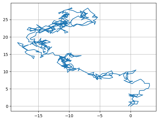
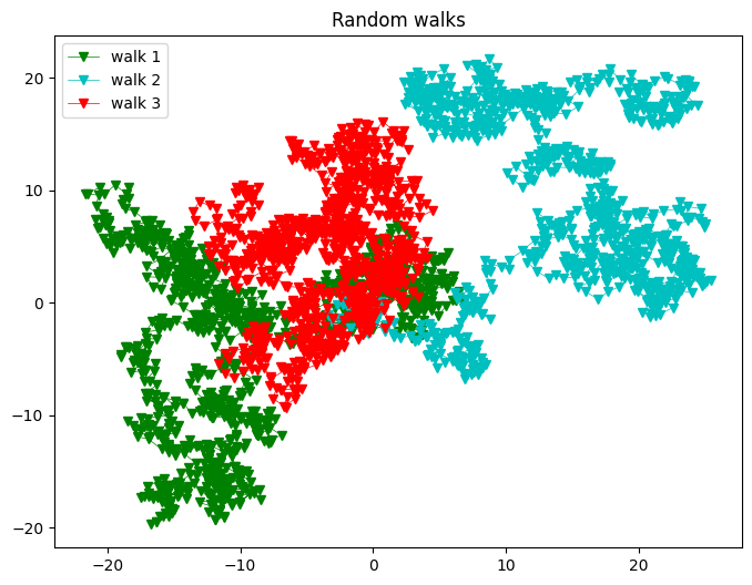
Start at the origin and take a 2D random walk. It is chosen values for \(\Delta x'\) and \(\Delta y'\) in the range [-1,1]. They are normalized so each step is of unit length.
np.random.uniform(1,-1)
-0.5980004387516238
#Initial positions
x0 = 0.
y0 = 0.
pos = [x0,y0]
#Number of random steps
N_steps = 1000
#Number of random walks
N_walks = 3


def Random_walk(N, x0=0,y0=0):
    pos=[x0,y0]

    x = [x0]
    y = [y0]

    #Generating random positions
    for i in range(1,N):
        x.append( np.random.uniform(1,-1) + x[i-1] )
        y.append( np.random.uniform(1,-1) + y[i-1] )

    return x, y
x,y=Random_walk(500)
plt.plot(x,y)
plt.grid()
colors = ('b', 'g', 'c', 'r', 'm', 'y', 'k')
axisNum = 0
plt.figure( figsize = (8,6) )

N_walks=3
#Plotting random walks
for j,c in zip( range(N_walks),colors):

    axisNum += 1
    x,y= Random_walk( N_steps )
    #If N_walks > repeat the colors
    color = colors[axisNum % len(colors)]
    plt.plot(x,y,"v-", color = color, lw= 0.5, label = "walk %d"%(j+1))


plt.title("Random walks")
plt.legend()
<matplotlib.legend.Legend at 0x7f7558571190>
8.5.2. #
Activity
Radioactive decay: Spontaneous decay is a natural process in which a particle, with no external stimulation, decays into other particles. Then, the total amount of particles in a sample decreases with time, so will the number of decays. The probability decay is constant per particle and is given byDetermin when radioactive decay looks like exponential decay and when it looks stochastic depending on the initial number of particles \(N(t)\) .For this, suposse that the decay rate is 0.3\(\times 10^6 s^{-1}\) . Make a logarithmic plot to show the results.
np.random.uniform(-15,15,(2,2))
array([[-11.81307268,  -4.22920799],
       [ -4.73925943,   7.47052026]])
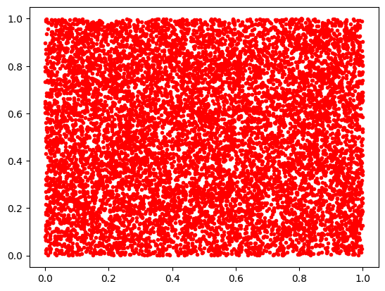
Espacio de parámetros aleatorios
N=10000
plt.plot(np.random.random(N),np.random.random(N),'r.')
[<matplotlib.lines.Line2D at 0x7f75586af880>]
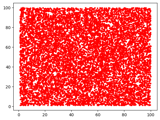
Hasta dos ordenes de magnitud
N=10000
plt.plot(np.random.uniform(1,100,N),np.random.uniform(1,100,N),'r.')
[<matplotlib.lines.Line2D at 0x7f75586206d0>]
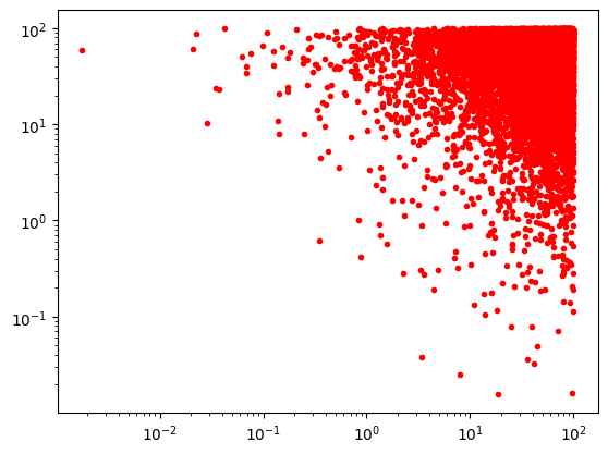
Varios ordenes de magnitud: \(10^{-4}\) a \(10^2\)
N=10000
plt.loglog(np.random.uniform(1E-4,1E2,N),np.random.uniform(1E-4,1E2,N),'r.')
[<matplotlib.lines.Line2D at 0x7f755860f880>]
\(x=10^{\log_{10}(x)}\)
10**np.log10(24.456)
24.455999999999996
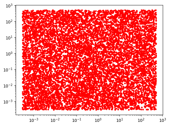
N=10000
xmin=3E-4;xmax=5E2
ymin=xmin;ymax=xmax
plt.loglog(  10**np.random.uniform(np.log10(xmin),np.log10(xmax),N),
             10**np.random.uniform(np.log10(ymin),np.log10(ymax),N),'r.')
[<matplotlib.lines.Line2D at 0x7f75582149a0>]
np.random.randint(1,100)
27
8.6. Appendix#
## Finding adjusting parameters
def Linear_least_square( x,y ):

    #Finding coefficients
    length = len(x)
    square_x = np.sum([x[i]**2 for i in xrange(length)])
    sum_xy = np.sum([x[i]*y[i] for i in xrange(length)])
    sum_x = np.sum(x)
    sum_y = np.sum(y)
    a0 = ( square_x*sum_y - sum_xy*sum_x ) / ( length*square_x  - sum_x**2 )
    a1 = ( length*sum_xy - sum_x*sum_y ) / ( length*square_x  - sum_x**2 )

    #Returning a_0 and a_1 coefficients
    return np.array([a0,a1])

#Line function adjusting the data set
def Line(a0,a1,x):
    return a0+a1*x
xrange=range
#========================================================
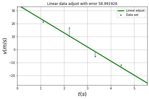
## Adjusting to a first order polynomy the data set v
#========================================================
#Setting figure
plt.figure( figsize = (8,5) )

#Time
t = np.array([ 0.,  1.11,  2.22,  3.33,  4.44, 5.55])

#Velocities measured for every time t[i]
v = np.array([33.10, 21.33, 16.57, -5.04, -11.74, -27.32])

#Making data adjust
a0, a1 = Linear_least_square( t,v )

#Finding error associated to linear approximation
E = np.sum([ ( v[i] - Line(a0,a1,t[i]) )**2  for i in xrange(len(t))])

#Plotting solution
plt.plot( t, Line(a0,a1,t), ".-", lw = 3.,color = "green",label="Lineal adjust" )
plt.plot( t, v, ".",color = "blue", label = "Data set" )
for i in xrange(len(t)):
    plt.plot(np.array([t[i],t[i]]), np.array([v[i],Line(a0,a1,t[i])]),"c-")

#Format of figure
plt.xlabel( "$t(s)$", fontsize = 18 )
plt.ylabel( "$v(m/s)$", fontsize = 18 )
plt.xlim( (t[0], t[-1]) )
plt.ylim( (v[-1], v[0]) )
plt.title("Linear data adjust with error %f"%E)
plt.legend()
plt.grid(1)
8.6.1. Activity #
http://scipy-cookbook.readthedocs.io/items/robust_regression.html
Using the next data set of a spring mass system, find the lineal adjust.