Notebooks#

Jupyter notebooks are a powerful web interface designed for interactive computing in multiple programming languages. Although it was initially designed for Python, its functionalities have quickly permeated other programming languagues. It have evolved from IPython, a replacement for the official Python shell in the console

It is worth mentioning the main author of IPython is Fernando Perez, a physicist graduate from the Universidad de Antioquia and currently Professor in University of California, Berkeley.

Official page

Features

Jupyter provides a rich architecture for interactive computing with:

Powerful interactive shells (terminal and Qt-based).
A browser-based notebook with support for code, text, mathematical expressions, inline plots and other rich media.
Support for interactive data visualization and use of GUI toolkits.
Flexible, embeddable interpreters to load into your own projects.
Easy to use, high performance tools for parallel computing.

Jupyter Notebooks#

Since 2011, Jupyter has incorporated a new funcionality called Notebooks. For

List item
List item

those who know notebooks of Mathematica® and SAGE this feature may be familiar.

Official page Jupyter Notebooks

The Jupyter Notebook (or Jupyter lab) is a web-based interactive computational environment where you can combine code execution, text, mathematics, plots and rich media into a single document. These notebooks are normal files that can be shared with colleagues, converted to other formats such as HTML or PDF, etc. You can share any publicly available notebook by using the GitHub viewer service which will render it as a static web page. This makes it easy to give your colleagues a document they can read immediately without having to install anything.

Cell phone installation

How to (step by step)#

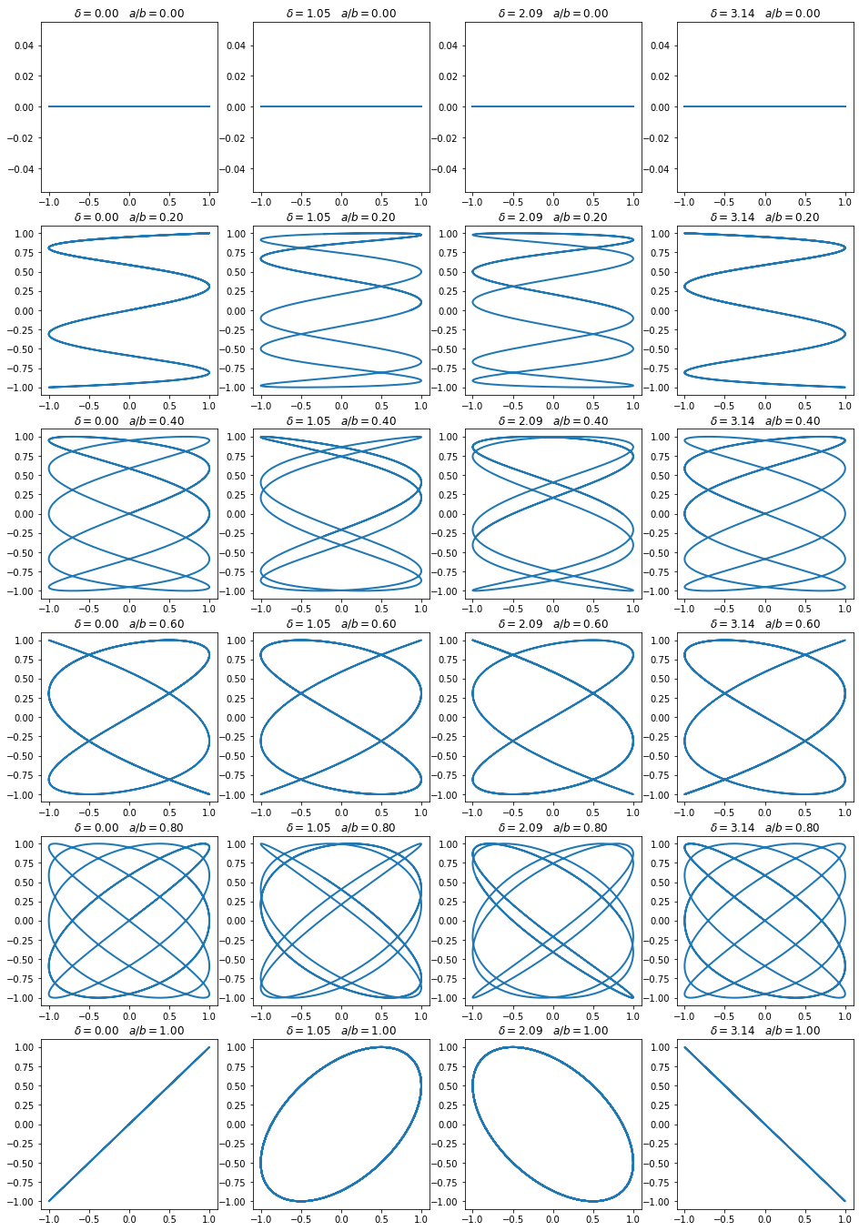
What is better than a step by step example when you want to introduce a new tool. Next it is shown a simple example of a IPython notebook for generating a family of Lissajous curves.

First, a suitable title for your notebook should be thought. For this, choose the style Heading 1 with # at the beggining.

Lissajous curves#

Then, a brief statement of the problem to solve should be done. For this, you can use the Markdown style. A useful reference for formatting markdown text can be found here.

Lissajous curves are a family of parametric two-dimensional curves normally obtained when solving multi-harmonic systems, like a mass-spring systems with two springs in each axis (x and y) or some circuit systems. The figures are described with the following equations:

You can use LaTex format in a Markdown cell, for this you must use double $

$x(t) = A\sin(a t +\delta)$

$y(t) = B\sin(b t)$

where $A$ and $B$ are the amplitudes along each axis, $a$ and $b$ the angular frequencies and $\delta$ the relative phase.

It is possible to embed figures from internet into a Markdown cell simply by writing:

![Some text](URL_to_figure)

Once established the problem, the first thing to do is to import all the libraries you should use for your calculations.

#This line is always necessary when you use matplotlib in a notebook, otherwise the figures will not appear.
%pylab inline
import matplotlib.pyplot as plt
import numpy as np

Populating the interactive namespace from numpy and matplotlib

You can create subsections and subsubsections using the styles Heading 2: with ##, and Heading 3: with ###

Plotting some curves#

Regarding coding, you can write Python code normally as if you were doing it in a text editor like emacs.

#Solutions
def Lissajous( t, A=1.0, B=1.0, a=1.0, b=1.0, delta=0.0 ):
    x = A*np.sin(a*t+delta)
    y = B*np.sin(b*t)
    return x, y

#Parameters to be sampled--------------------
#delta
Ndelta = 4   #Number of delta parameters
Delta = np.linspace(0,np.pi,Ndelta)
#Ratio c=a/b
Nratio = 6  #Number of c parameters
C = np.linspace(0,1,Nratio)
#Time array
T = np.linspace(0,40,1000)

#Initializing plotting environment
plt.figure( figsize=(4*Ndelta, 4*Nratio) )
plt.subplot( Nratio, Ndelta, 1 )
plt.plot()
#Sweeping all figures
for i in range( Ndelta ):
    for j in range( Nratio ):
        #Creating a subfigure with the current delta and ratio c
        plt.subplot( Nratio, Ndelta, j*Ndelta+i+1 )
        #Plotting this Lissajous curve
        X, Y = Lissajous( T, b=C[j], delta=Delta[i] )
        plt.title( "$\delta=$%1.2f\t$a/b=$%1.2f"%(Delta[i],C[j]) )
        plt.plot( X, Y, linewidth=2 )

/usr/local/lib/python3.7/dist-packages/ipykernel_launcher.py:19: MatplotlibDeprecationWarning: Adding an axes using the same arguments as a previous axes currently reuses the earlier instance.  In a future version, a new instance will always be created and returned.  Meanwhile, this warning can be suppressed, and the future behavior ensured, by passing a unique label to each axes instance.

References#

http://en.wikipedia.org/wiki/Lissajous_curve

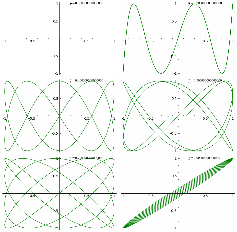
For this activity, you should obtain something like this.

Viewing your notebook online#

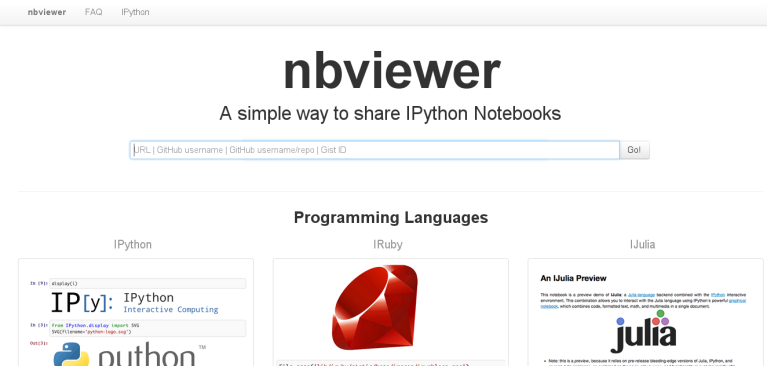
Once you have a notebook, you can upload it in some online storage service like Dropbox or Google drive or some repository service like GitHub or GitLab. In both GitHub and GitLab the notebooks are automatically displayed in their web interfaces. Also, you can put the link of your notebook directly into the IPython Notebook Viewer.

from IPython.display import display, Markdown, Latex, Image 
Image(filename='./figures/nbviewer.png')

display(Markdown('*some markdown* $\phi={}$'.format(2)))

some markdown $\phi=2$

Computational Methods

Notebooks

Contents